Querying streams with SQL

Note	This lab assumes that the From Edge to Streams Processing lab has been completed.

In this workshop you will use SQL Stream Builder to query and manipulate data streams using SQL language. SQL Stream Builder is a powerful service that enables you to create Flink jobs without having to write Java/Scala code.

Labs summary

Step 1 - Create a Data Source
Step 2 - Create a Source Virtual Table for a topic with JSON messages
Step 3 - Run a simple query
Step 4 - Computing and storing aggregation results

Introduction

In this lab, and the subsequent ones, we will use the iot topic created and populated in previous labs and contains a datastream of computer performance data points.

So let’s start with a straightforward goal: to query the contents of the iot topic using SQL to examine the data that is being streamed.

Albeit simple, this task will show the ease of use and power of SQL Stream Builder (SSB).

Lab 1 - Create a Data Source for IoT Topic

Before we can start querying data from Kafka topics we need to register the Kafka clusters as data sources in SSB.

On the landing page or Cloudera Manager console, click on the Cloudera logo at the top-left corner to ensure you are at the home page and then click on the SQL Stream Builder service.
Click on the SQLStreamBuilder Console link to open the SSB UI.
On the logon screen, authenticate with user admin and password Supersecret1
Click on Data Providers you will notice that SSB already has a Kafka cluster registered as a data source, named CDP Kafka. This source is created automatically for SSB when it is installed on a cluster that also has a Kafka service:
You can use this screen to add other external Kafka clusters as data sources to SSB.

Lab 2 - Create a Source Virtual Table for a topic with JSON messages

Now we can map the iot topic to a virtual table that we can reference in our query. Virtual Tables on SSB are a way to associate a Kafka topic with a schema so that we can use that as a table in our queries.

We will use a Source Virtual Table now to read from the topic. Later we will look into Sink Virtual Tables to write data to Kafka.

To create our first Source Virtual Table, click on Console (on the left bar) > Tables > Add table > Apache Kafka.

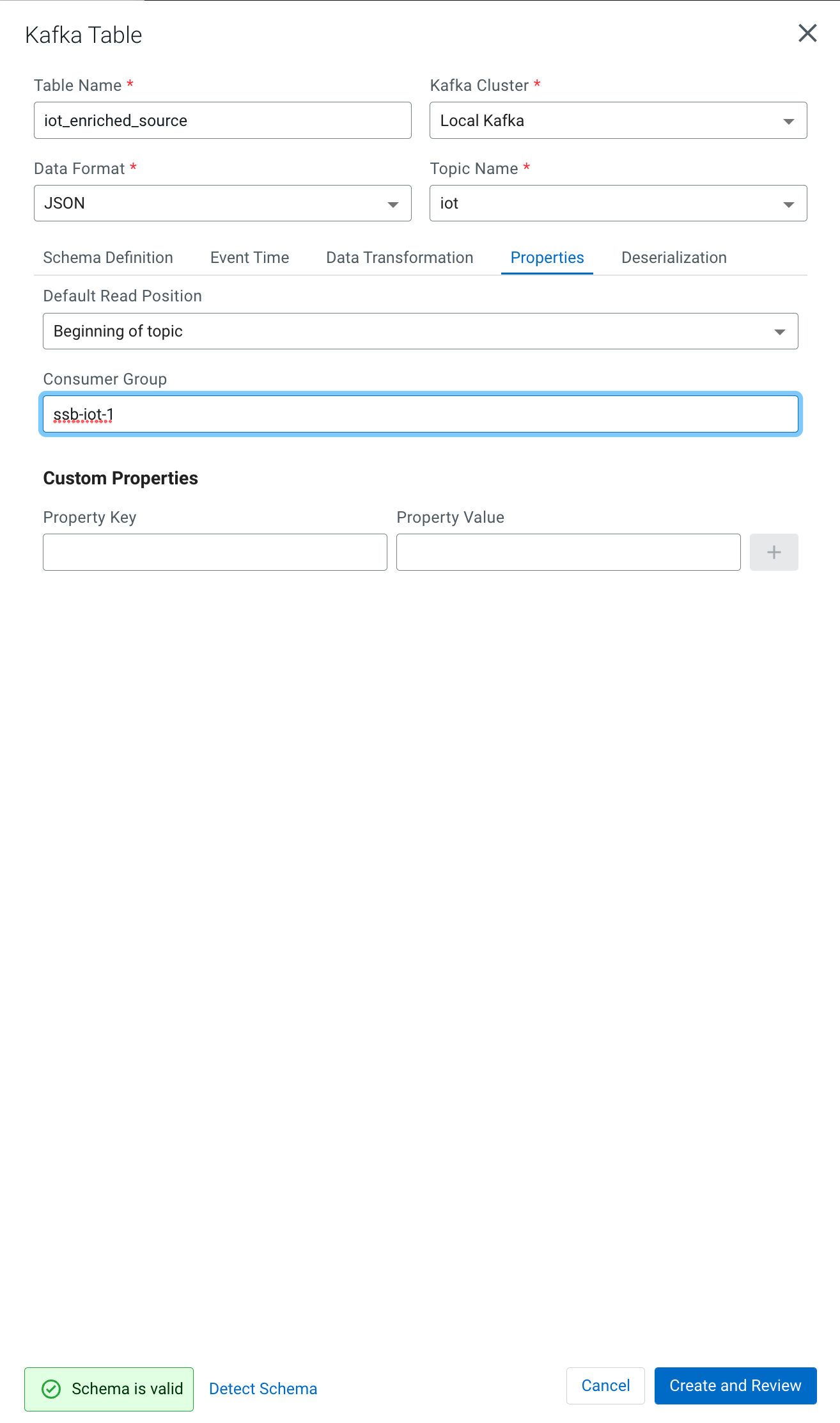
On the Kafka Source window, enter the following information:

Virtual table name: iot_enriched_source
Kafka Cluster:      CDP Kafka
Topic Name:         iot
Data Format:        JSON

Ensure the Schema tab is selected. Scroll to the bottom of the tab and click Detect Schema. SSB will take a sample of the data flowing through the topic and will infer the schema used to parse the content. Alternatively you could also specify the schema in this tab.
Click on the Event Time tab, define your time handling. You can specify Watermark Definitions when adding a Kafka table. Watermarks use an event time attribute and have a watermark strategy, and can be used for various time-based operations.

The Event Time tab provides the following properties to configure the event time field and watermark for the Kafka stream:
- Input Timestamp Column: name of the timestamp column in the Kafka table from where the event time column is mapped. If you wanna use a colume from the event message you have to unselect the box Use Kafka Timestamp first.
- Event Time Column: new name of the timestamp column where the watermarks are going to be mapped
- Watermark seconds : number of seconds used in the watermark strategy. The watermark is defined by the current event timestamp minus this value.
  Input Timestamp Column: sensor_ts Event Time Column: event_ts Watermark Seconds: 3
If we need to manipulate the source data to fix, cleanse or convert some values, we can define transformations for the data source to perform those changes. These transformations are defined in Javascript.

The serialized record read from Kafka is provided to the Javascript code in the record.value variable. The last command of the transformation must return the serialized content of the modified record.

The sensor_0 data in the iot topic has a pressure expressed in micro-pascal. Let’s say we need the value in pascal scale. Let’s write a transformation to perform that conversion for us at the source.

Click on the Transformations tab and enter the following code in the Code field:
```
// Kafka payload (record value JSON deserialized to JavaScript object)
var payload = JSON.parse(record.value);
payload['sensor_0'] = Math.round(payload.sensor_0 * 1000);
payload['sensor_ts'] = Math.round(payload.sensor_ts / 1000);
JSON.stringify(payload);
```
Click on the Properties tab, enter the following value for the Consumer Group property and click Save changes.
```
Consumer Group: ssb-iot-1
```
Click on "Create and Review"

Click on "Keep" to save the virtual table

Note

Setting the Consumer Group properties for a virtual table will ensure that if you stop a query and restart it later, the second query execute will continue to read the data from the point where the first query stopped, without skipping data. However, if multiple queries use the same virtual table, setting this property will effectively distribute the data across the queries so that each record is only read by a single query. If you want to share a virtual table with multiple distinct queries, ensure that the Consumer Group property is unset.

Lab 3 - Run a simple query

We have now all that we need to run our first query in SSB. We want to simply query the raw contents of topic to ensure that the everything is working correctly before we proceed to do more complex things.

If your environment is healthy and all the steps from previous labs were completed correctly you should be able to visualize the data with the steps below.

On the SSB UI, click on Console (on the left bar) *> Compose add the following query:
```
select count(*)
from iot_enriched_source
```
Set a SQL Job Name for your job or use the random name provided.
Do not add a Sink Virtual Table.
Click Execute
Scroll to the bottom of the page and you will see the log messages generated by your query execution.
Change the SQL query to:
```
select *
from iot_enriched_source
```
"Restart" and after a few seconds the SQL Console will start showing the results of the query coming from the iot topic.

The data displayed on the screen is only a sample of the data returned by the query, not the full data. The column on the right shows the previously defined Event Time
Well done! Let’s increase the level of difficulty and replace the existing SQL with the HELLO WORLD in streaming and counting the events by sensor_id - standard SQL with GROUP BY and COUNT.
```
select sensor_id,
  count(*) as sensorCount
from iot_enriched_source
group by sensor_id
```

After editing SQL - click on Restart

Warning

Make sure to stop your queries to release all resources once you finish this lab. You can double-check that all queries/jobs have been stopped by clicking on the SQL Jobs tab. If any jobs are still running, you can stop them from that page.

Lab 4 - Computing and storing aggregation results

This query will compute aggregates over 30-seconds windows that slide forward every second. For a specific sensor value in the record (sensor_6) it computes the following aggregations for each window:

Number of events received
Sum of the sensor_6 value for all the events
Average of the sensor_6 value across all the events
Min and max values of the sensor_6 field
Number of events for which the sensor_6 value exceeds 70

Let’s first create a topic (sensor6_stats) where to publish our aggregation results:

Navigate to the SMM UI (Cloudera Manager > SMM service > Streams Messaging Manager Web UI).
On the SMM UI, click the Topics tab ().
Click the Add New button.
Enter the following details for the topic and click Save when ready:
1. Topic name: sensor6_stats
2. Partitions: 10
3. Availability: Low
4. Cleanup Policy: delete

On the SSB UI:

Click on Console (on the left bar) > Compose > SQL
Create new job, enter e.g. Sensor6Stats for the SQL Job Name field.

In the SQL box type the query shown below.

SELECT
  sensor_id as device_id,
  HOP_END(event_ts, INTERVAL '1' SECOND, INTERVAL '30' SECOND) as windowEnd,
  count(*) as sensorCount,
  sum(sensor_6) as sensorSum,
  avg(cast(sensor_6 as float)) as sensorAverage,
  min(sensor_6) as sensorMin,
  max(sensor_6) as sensorMax,
  sum(case when sensor_6 > 70 then 1 else 0 end) as sensorGreaterThan60
FROM iot_enriched_source
GROUP BY
  sensor_id,
  HOP(event_ts, INTERVAL '1' SECOND, INTERVAL '30' SECOND);

Before we can publish events to the new created topic we have to execute this query to build the template.
Next the sensor6_stats_sink table must be created in SSB, mapping it to the sensor6_stats Kafka topic.
Since we want the topic format to be JSON, click on Templates > CDP Kafka > JSON.
This will prepend a CREATE TABLE DDL to the SQL script to create a table that matches the structure of your query! Adjusted the name e.g. sensor6_stats_sink
Most of the table properties are already filled in for you. But there’s one you must edit before you execute the statement: the topic property.

Edit the DDL statement and replace the … value of the topic property with the actual topic name: sensor6_stats.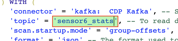
Click Execute to create the sink table

Copy & past the SQL box again, this time including a`sensor6_stats_sink` statement on top.

INSERT INTO sensor6_stats_sink
SELECT
  sensor_id as device_id,
  HOP_END(event_ts, INTERVAL '1' SECOND, INTERVAL '30' SECOND) as windowEnd,
  count(*) as sensorCount,
  sum(sensor_6) as sensorSum,
  avg(cast(sensor_6 as float)) as sensorAverage,
  min(sensor_6) as sensorMin,
  max(sensor_6) as sensorMax,
  sum(case when sensor_6 > 70 then 1 else 0 end) as sensorGreaterThan60
FROM iot_enriched_source
GROUP BY
  sensor_id,
  HOP(event_ts, INTERVAL '1' SECOND, INTERVAL '30' SECOND);

Let’s query the sensor6_stats topic to examine the data that is being written to it. Create a new job via + New Job

Note
The sensor6_stats job will continue to run in the background. You can monitor and manage it through the SQL Jobs page.
Let’s query the sensor6_stats table to examine the data that is being written to it. First we need to define a Source Table associated with the sensor6_stats topic.
1. Click on Console (on the left bar) > Apache Kafka
2. On the Kafka Source window, enter the following information and click Save changes:
  
  Virtual table name: sensor6_stats_source Kafka Cluster: CDP Kafka Topic Name: sensor6_stats Data Format: JSON
1. Click on Detect Schema and wait for the schema to be updated.
2. Click Save changes.
Click on Console (on the left bar) to refresh the screen and clear the SQL Compose field, which may still show the running aggregation job.

Note that the job will continue to run in the background and you can continue to monitor it through the Job Logs page.
Enter the following query in the SQL field and execute it:
```
SELECT *
FROM sensor6_stats_source
```

After a few seconds you should see the contents of the sensor6_stats topic displayed on the screen:

Warning

Make sure to stop your queries to release all resources once you finish. CSA CE is limited to a few worker tasks. You can double-check that all queries/jobs have been stopped by clicking on the SQL Jobs tab. If any jobs are still running, you can stop them from that page.

Click on the Flink Dashboard link to open the job’s page on the dashboard. Navigate the dashboard pages to explore details and metrics of the job execution.

Conclusion

We have now taken data from one topic, calculated aggregated results and written these to another topic. In order to validate that this was successful we have selected the result with an independent select query.

Provide feedback

Saved searches

Use saved searches to filter your results more quickly

sql_stream_builder_lite.adoc

sql_stream_builder_lite.adoc

Querying streams with SQL

Labs summary

Introduction

Lab 1 - Create a Data Source for IoT Topic

Lab 2 - Create a Source Virtual Table for a topic with JSON messages

Lab 3 - Run a simple query

Lab 4 - Computing and storing aggregation results

Conclusion

Files

sql_stream_builder_lite.adoc

Latest commit

History

sql_stream_builder_lite.adoc

File metadata and controls

Querying streams with SQL

Labs summary

Introduction

Lab 1 - Create a Data Source for IoT Topic

Lab 2 - Create a Source Virtual Table for a topic with JSON messages

Lab 3 - Run a simple query

Lab 4 - Computing and storing aggregation results

Conclusion